
A Brief Introduction to the Spectropolarimetry of Supernovae
Intro
Spectropolarimetry is a great tool that allows us to infer 3 dimensional information about unresolved supernova ejecta. I hope this brief intro will help those that are just starting, or maybe people who have found themselves a bit confused when reading a paper that mentions spectropolarimetry. I’ve basically created the resource and pictures I wish I had access to when I started. You should also check out the Annual Review by Wang & Wheeler (2008).
What is polarisation?
It’s a general property of transverse waves which characterises the orientation of oscillations. In the case of E-M radiation, it describes the orientation of the electric vector.
There are two main types of polarisation: linear and circular. In the case of linear polarisation, the electric vector oscillates in one direction, and in the case of circular polarisation the direction of the electric vector rotates in the plane orthogonal to the direction of propagation (see Figure 1).
Elliptical polarisation is a mixture of linear and circular polarisation. In the context of supernovae we’re only interested in linear polarisation so that is what we will focus on for the rest of this introduction.
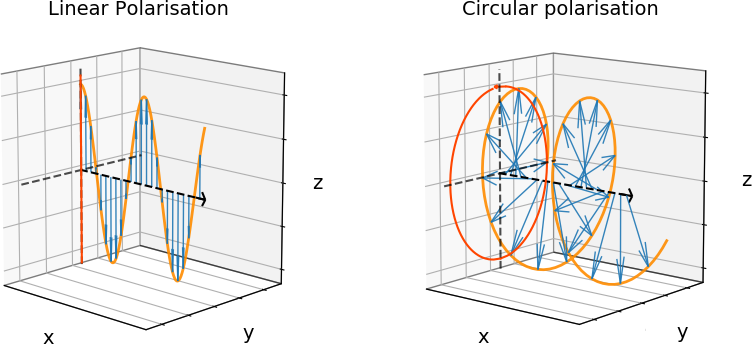
Figure 1: Schematic of linear and circular polarisation. The light is propagating in the z direction, the blue arrows show the direction of the oscillation of the electric vector (yellow). In dark orange the projection of the electric vector oscillation is shown.
Quantifying polarisation
The Stokes Parameters
To quantify the direction in which the electric vector is oscillating we use the Stokes parameters. They are pseudo-vectors, meaning that their 0 degree and 180 degree direction are the same. If you look at the left panel of Figure 1 this is easy to picture: It doesn’t matter if the blue arrow points up or down, it is still aligned with the direction showed by the dark orange projection.
There are 4 Stokes Parameters: I, Q, U, V.
I is the total intensity of your light (the flux in spectroscopy)
Q and U define linear polarisation
V defines circular polarisation
As mentioned above, we focus on linear polarisation (Q and U). By convention, +Q points in the 0 degree North-South direction. Because Stokes Parameters are pseudo-vectors, -Q is oriented 90 degrees from +Q. Stokes U is oriented 45 degrees from +Q (anti-clockwise), and -U 135 degrees. Adding a +Q (+U) and -Q (-U) vector of the same amplitude results in zero polarisation. These concepts can be visualised in Figure 2.

Figure 2: Visualisation of the Stokes Parameters
It is very common for people to use normalised Stokes parameters: q=Q/I and u=U/I with units of percent (i.e. a percentage of the total flux). Note that the notation q and u for normalised stokes parameters is common but not unique. Some papers will still use capital Q and U, but they are most likely talking about normalised Stokes; if in doubt, check their Methods or Observations section.
Degree of Polarisation and Polarisation Angle
Stokes parameters are often visualised on the q-u plane, where the x-y axis correspond to the q and u amplitudes (right panel — Figure 3). This is like taking the q-u directions as defined on the plane of the sky, unfolding them so they span 360 degrees (instead of 180) and rotating the whole thing clockwise by 90 degrees (compare the axes on the left and right panel of Figure 3). As we’ll see this is a very useful and informative way of plotting the Stokes parameters.
Now, if we take a polarimetric data point with a value of q and a value of u and plot it on the q-u plane (see the big grey blob in Figure 3 — right panel), we can define the degree of polarisation, as being the distance from our data point to the origin. The polarisation angle (P.A.) corresponds to the angle on the sky between the direction of oscillation of the electric field and our zero point (North-South direction. As you can see on Figure 3, the angle between our data point and the q-axis is arctan(u/q), and it is also 2x the polarisation angle since the q-u plane is an unfolded version of the Stokes vectors as defined on the plane of the sky.
For quick reference, here are the formulae for p and P.A.
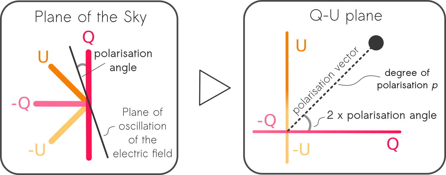
Figure 3: From the plane of the sky to the q-u plane.

P and P.A.
q and u are the normalised Stokes Parameters, p is the degree of polarisation and theta is the polarisation angle (P.A.)
Where does it come from?
Thomson scattering
Thomson scattering is the scattering of electro-magnetic radiation by a free charged particle, in the limit where the wavelength of the radiation is much greater than Compton wavelength of the particle (h/mc) — otherwise it is plain old Compton scattering. It is wavelength independent.
In the context of supernovae (and the winds of Wolf-Rayet stars), electron scattering is the dominant form of opacity, and often you’ll see the terms Thomson Scattering and Electron Scattering used interchangeably.
A photon that has undergone Thomson scattering will be polarised perpendicularly to the plane of scattering, which is defined as containing the incident and outgoing ray (Chandrasekhar 1960).
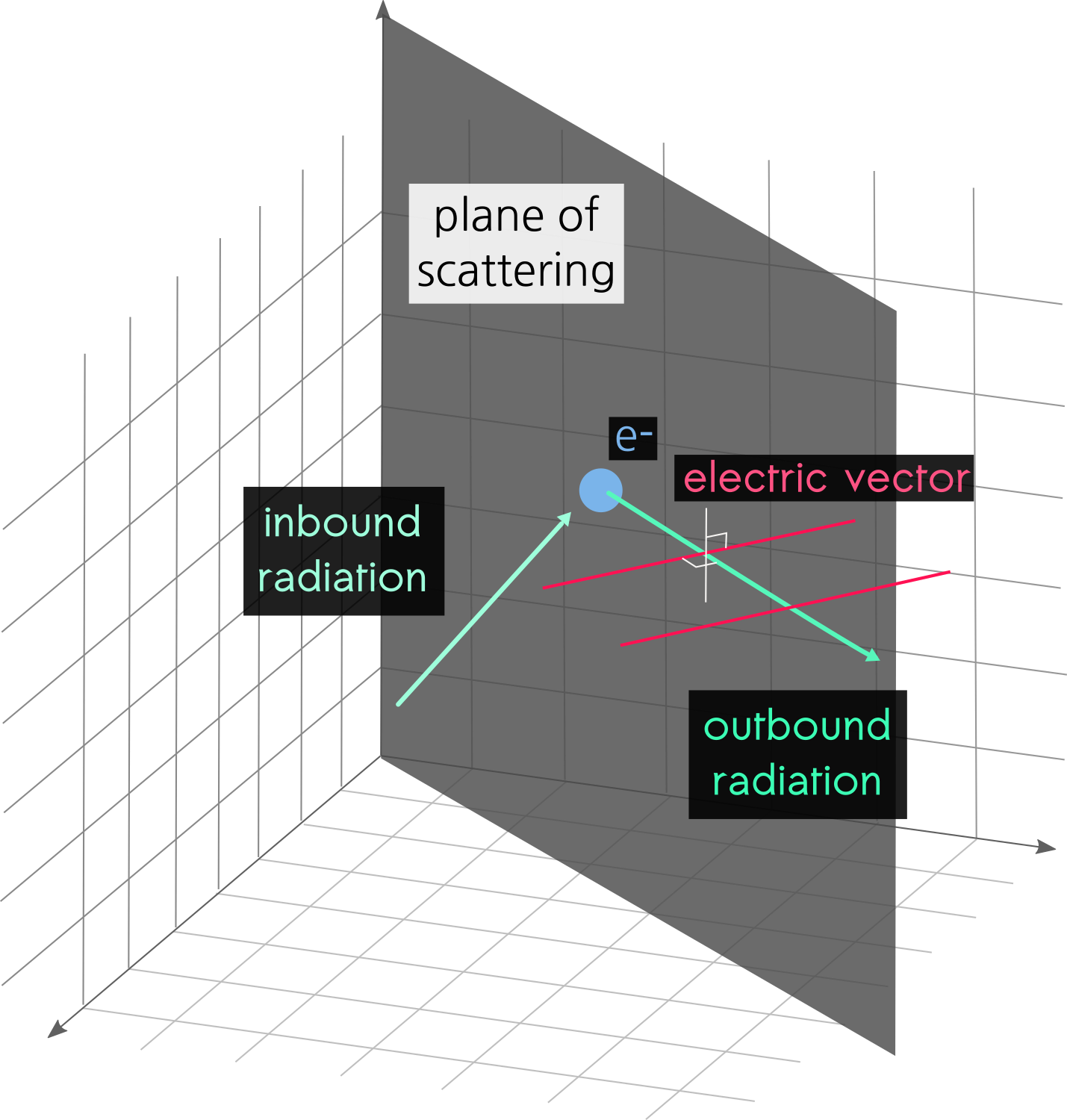
ELECTRON SCATTERING
Electron scattering is a form of Thomson scattering. It polarises the light perpendicularly to the plane of scattering, which is defined as the plane containing the inbound and outbound photons.
Polarisation in an electron dominated photosphere
Now let’s consider a point on the edge of the photodisc (projection of the photosphere on the plane of the sky) . The incoming radiation — see dotted green arrows in Figure 4 — will come from all direction beneath that point. On average their vertical components cancel out, and the dominant direction of the incoming radiation comes from the centre — the solid green arrow. Now, since we only care about the light that we get to see, the outbound radiation comes out of the page — or screen — towards you. The preferential direction of the polarisation will be perpendicular to the plane of scattering defined by the inbound and outbound radiation, and will therefore be tangential to the photosphere at the point of scattering.

Figure 4: Polarisation at the edge of the photosphere.

Figure 5: The polarisation at the centre of the photosphere is zero.
If we now consider the point at the centre of the photodisc, the inbound and outbound rays are in-line (see Figure 5). Consequently these two rays can define an infinity of planes of scattering, instead of constraining one. The light radiating from this point is not preferentially polarised.
The two cases described above are limiting cases.
On the whole:
The light is polarised tangentially to the photosphere. The amplitude of the polarisation is zero in the centre and increases as you move towards the limb, where it is maximised.
Polarisation and Asymmetry
Since supernovae are very distant they are unresolved and therefore the observed polarisation will be a sum the polarisation components across the whole photodisc. Let’s have a look at a few basic configurations.
Polarisation of a spherical photosphere

Figure 6: The q-u vectors of a spherical photosphere cancel out completely.
First let’s consider the simplest case: A circular photodisc.
Figure 6 illustrates how the polarisation is distributed, with polarisation vectors tangential to the photosphere of increasing amplitude towards the limb. As we can see the Q and -Q vectors all have the same amplitude — same goes for U. Consequently the Stokes parameters cancel out completely when we integrate over the whole photodisc.
Polarisation of aspherical geometries
Now let’s look at aspherical cases, were the cancellation of the Stokes parameter is incomplete. So far we’ve only talked about the photosphere, but there is a lot going on in the ejecta above the photosphere that can also cause departure from sphericity. Also, polarisation probes deviations from sphericity in both the structure of the photosphere and the direction and focus of the radiation reaching the photosphere. All of this leads to three classical base cases:
(i) Aspherical electron distributions, such as ellipsoidal photosphere, resulting in continuum polarisation (e.g. Hoflich, 1991).
(ii) Partial obscuration of the underlying Thomson-scattering photosphere leading to line polarisation (e.g. Kasen et al. 2003).
(iii) Asymmetric energy input, e.g. heating by off-centre radioactive decay (Hoflich, 1995).
This simple cases lead to axial geometry, and they are illustrated in Figure 7 below.

Figure 7: Illustrations of case (i), (ii) and (iii). The photosphere is shown in black, the absorption region is shown in blue and the additional energy input is shown in yellow. We only show Stoke Q for clarity since the U components cancel out completely in these idealised cases. The dashed grey line shows the axis of symmetry.
Obviously these situations can be compounded: you can (and will) get absorbing line forming regions in front of an ellipsoidal photosphere. These situations would break axial geometry, and give really interesting features which we discuss further down.
From 2D to 3D: Homologous expansion and velocity slices
All the examples above showed how polarisation showed asymmetry but as you may have noticed when we integrate our Stokes parameters we do it over a projection of our eject on the plane of the sky — so in 2 dimensions.

Figure 8: Velocity slices (represented by the vertical blue lines) and P Cygni profile.
So where does the third dimension come from?
A few hours to a few days after explosion, the ejecta of supernovae can be assumed to be in homologous expansion: In other words, the fast material is found in the outer parts of the ejecta and the slow material is in the interior — radius = velocity x time. Therefore, the 3D geometry of the envelope does not change over time (at least not on the timescales we consider), and variations in the degree of polarisation p, and Stokes q, u are the result of the photosphere receding in a hydro-dynamically inert structure. Furthermore, to combined effect of homologous expansion and Doppler shift across P Cygni pro files means that different wavelengths across a line feature will probe different velocity slices (see Figure 8 — each slice is a flat projection of the photosphere on the sky). Investigating the polarisation at different wavelengths allows us to probe the third dimension: depth.
The features in polarisation data
Now that we’ve discussed the basics of where polarisation comes from and how it is related to the geometry of the ejecta, it would be worth taking a look at what kind of features we expect and see in our data.
Inverse P Cygni Profiles
P Cygni profiles are ubiquitous in the early spectra of supernovae. As shown in the previous section (see Figure 8), the blue shifted absorption component probes successive velocity slices or depths in the ejecta. It was predicted by McCall (1984) that the absorption component of P Cygni profiles would be associated with polarisation peaks as the line forming region would mainly block light from the central — less polarised — region.
The emission component of the P Cygni profile around the rest wavelength and redward, is due to the scattering of photons into our line of sight by ions or atoms in the ejecta. This is done via resonant scattering which is a non-polarising process. Consequently the polarised continuum will be diluted by the non-polarised flux in emission, causing a dip (see Figure 9).

Figure 9: Polarisation (purple) associated with He I 5876 and H alpha in the type IIb SN 2011hs around maximum light. The flux spectrum is shown in dark grey.
q-u plots: dominant axis and loops
The q-u plot is one of the pillars of supernova spectropolarimetric studies because it can deliver so much information about the geometry of the ejecta. It also usually shows the wavelength component as a colour bar, to help link the polarisation to the spectral information. This helps highlight behaviour changes associated with specific lines.
Generally speaking, there are two main features that people will look for: A dominant axis and loops.

Q-U PLOT
Polarisation data plotted on the q-u plane, often showing wavelength in a colour bar

DOMINANT AXIS
Axis of preferred alignment present in some data sets. Marker of axial symmetry.
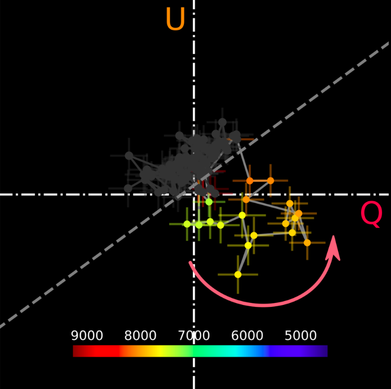
Q-U LOOPS
They are the rotation of the polarisation angle sometimes associated with the absorption components of strong lines. (In this case, the calcium infra-red triplet)
If we consider the case of a photosphere with axial geometry (e.g. case (i) and (iii) see Figure 7) and fully symmetry line forming regions, such that they induce no polarisation. Then, the polarisation angle (P.A.) will be the same across the spectrum, but the degree of polarisation (p) may vary due to dilution effects, optical depths… This single P.A. and variable p result in a line on the q-u plane. Real supernova ejecta are not such ideal cases, but an preferred alignment onto a Dominant Axis is a marker of global axial symmetry (see recent models of Tanaka+2017 - which include bipolar configurations).
Sometimes, the polarisation data associated with specific spectral lines shows rotations in P.A. with wavelength. When plotted on the q-u plot, these will manifest as loops. They are the result of a departure from axial symmetry. This departure can occur on a global scale, for example the presence of an off-axis energy source in an ellipsoidal ejecta — case (i) + (iii) — or it can be line specific, such as partial blocking of an ellipsoidal photosphere — case (i) + (ii). Being able to isolate a possible cause for this departure, and whether it is on a large or smaller scale, requires a careful analysis of the data on a case by case basis.
The animation in Figure 10 shows how the loop forms as we move across the absorption component of the P Cygni profile.
Figure 10: Animated q-u plot of the calcium triplet of SN 2014ad
Note that significant departures from the dominant axis do not always form loops but are still markers of a break of axial symmetry.
Continuum Vs Line polarisation
In most papers, there will be mentions of continuum polarisation and line polarisation. Continuum polarisation is caused by the large scale asymmetries of the photosphere. Line polarisation on the other hand can be due to either line specific phenomena (e.g. clumps!!) or global effects (e.g. shape of the photosphere, off-centre energy sources). Careful analysis of the polarisation of different lines, comparison to the continuum, and tracking the evolution over time can help us identify the cause of the polarisation.
30 years of CCSN SpecPol in 3 minutes
This is a very quick — non exhaustive!! — summary of some of the main results obtained from spectropolarimetric analysis of Core Collapse Supernovae.
Virtually all SNe show asymmetry.
Type II-P tend to show little to no polarisation at early times. A jump in polarisation is seen as the lightcurve comes off the plateau. This sudden increase in polarisation is interpreted as a manifestation of the photosphere receding through the outer hydrogen envelope, revealing an inner more aspherical core. (e.g. see SN 1987A, Jeffery 1991 — SN 2004dj, Leonard et al., 2006)
Polarisation changes when the photosphere transitions from the hydrogen envelope to deeper layers can also be seen in some type IIb SNe (e.g. SN 1993J, Tran et al. 1997 — SN 2001ig, Maund et al. 2007). This is not universal though, SN 2008ax showed high line polarisation at early times (Chornock et al. 2011), SN 2011dh had a roughly constant continuum polarisation as the spectrum showed the transition to the helium layer and a subsequent decrease in polarisation. A similar behaviour was also seen in SN 2011hs (Stevance et al. 2019). Line and continuum polarisation analysis in SN 2011dh and SN 2011hs revealed the potential presence of Nickel plumes.
Type Ib/c SNe show diversity in the degree of polarisation observed, with the case of SN 1997X (Wang et al., 2001) exhibiting p at least 4 percent, whilst other examples such as SN 2005bf or SN 2008D showed lower continuum levels — but still higher than in type II-P at early days (Tanaka et al., 2009, Maund et al., 2009). The spectropolarimetric analysis of SN 2005bf and SN 2008D suggested the presence of jets.
I don’t know enough about the type Ias to even attempt to include them. If you do and would like to contribute, feel free to get in touch.
Summary
Spectropolarimetry is a very useful technique that can reveal the 3 dimensional geometry of unresolved ejecta.
Linear polarisation is defined by the Stokes parameters Q (0 degrees North) and U (45 degrees from Q - anti-clockwise).
Polarisation in supernovae and Wolf-Rayet star winds arises from electron scattering, which preferentially polarises the light tangentially to the photosphere (or point of last scattering).
Since the ejecta is unresolved, we must sum all the polarisation components, and spherical geometries will lead to complete cancellation of the Stokes parameters.
Aspherical geometries yield a polarisation excess that can be measured.
A dominant axis on the q-u plot is a marker of axial symmetry.
Departures from the dominant axis indicate a departure from axial symmetry.
Continuum polarisation tracks global geometry effects, whilst line polarisation can be affected both by line specific and large scale geometries.
All SNe are asymmetric.